Evolution of a salesman: Genetic Algo for Python
Introduction
The problem
In this article, we’ll be using a GA to find a solution to the traveling salesman problem (TSP). The TSP is described as follows:
“Given a list of cities and the distances between each pair of cities, what is the shortest possible route that visits each city and returns to the origin city?”
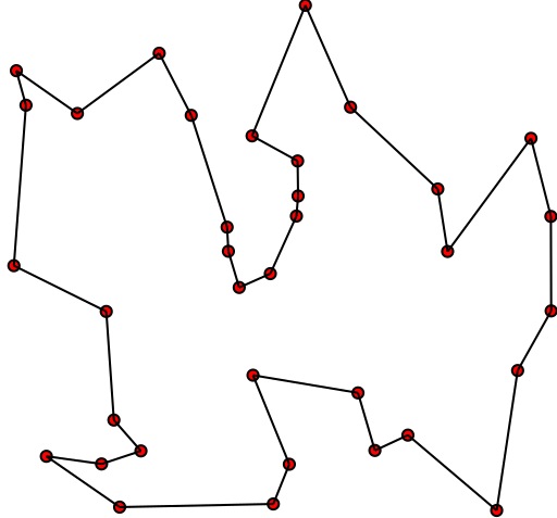
Illustration of a potential solution to the TSP (By Xypron [Public domain], from Wikimedia Commons)
Given this, there are two important rules to keep in mind:
- Each city needs to be visited exactly one time
- We must return to the starting city, so our total distance needs to be calculated accordingly
The approach
Let’s start with a few definitions, rephrased in the context of the TSP:
- Gene: a city (represented as (x, y) coordinates)
- Individual (aka “chromosome”): a single route satisfying the conditions above
- Population: a collection of possible routes (i.e., collection of individuals)
- Parents: two routes that are combined to create a new route
- Mating pool: a collection of parents that are used to create our next population (thus creating the next generation of routes)
- Fitness: a function that tells us how good each route is (in our case, how short the distance is)
- Mutation: a way to introduce variation in our population by randomly swapping two cities in a route
- Elitism: a way to carry the best individuals into the next generation
Our GA will proceed in the following steps:
-
- Create the population
-
- Determine fitness
-
- Select the mating pool
-
- Breed
-
- Mutate
-
- Repeat
Now, let’s see this in action.
Building our genetic algorithm
While each part of our GA is built from scratch, we’ll use a few standard packages to make things easier:
import numpy as np, random, operator, pandas as pd, matplotlib.pyplot as plt
Create two classes: City and Fitness
We first create a City class that will allow us to create and handle our cities. These are simply our (x, y) coordinates. Within the City class, we add a distance calculation (making use of the Pythagorean theorem) in line 6 and a cleaner way to output the cities as coordinates with __repr__ in line 12.
class City:
    def __init__(self, x, y):
        self.x = x
        self.y = y

    def distance(self, city):
        xDis = abs(self.x - city.x)
        yDis = abs(self.y - city.y)
        distance = np.sqrt((xDis ** 2) + (yDis ** 2))
        return distance

    def __repr__(self):
        return "(" + str(self.x) + "," + str(self.y) + ")"
We’ll also create a Fitness class. In our case, we’ll treat the fitness as the inverse of the route distance. We want to minimize route distance, so a larger fitness score is better. Based on Rule #2, we need to start and end at the same place, so this extra calculation is accounted for in line 13 of the distance calculation.
class Fitness:
    def __init__(self, route):
        self.route = route
        self.distance = 0
        self.fitness= 0.0

    def routeDistance(self):
        if self.distance ==0:
            pathDistance = 0
            for i in range(0, len(self.route)):
                fromCity = self.route[i]
                toCity = None
                if i + 1 < len(self.route):
                    toCity = self.route[i + 1]
                else:
                    toCity = self.route[0]
                pathDistance += fromCity.distance(toCity)
            self.distance = pathDistance
        return self.distance

    def routeFitness(self):
        if self.fitness == 0:
            self.fitness = 1 / float(self.routeDistance())
        return self.fitness
Create the population
We now can make our initial population (aka first generation). To do so, we need a way to create a function that produces routes that satisfy our conditions (Note: we’ll create our list of cities when we actually run the GA at the end of the tutorial). To create an individual, we randomly select the order in which we visit each city:
def createRoute(cityList):
    route = random.sample(cityList, len(cityList))
    return route
This produces one individual, but we want a full population, so let’s do that in our next function. This is as simple as looping through the createRoute function until we have as many routes as we want for our population.
def initialPopulation(popSize, cityList):
    population = []

    for i in range(0, popSize):
        population.append(createRoute(cityList))
    return population
- Note: we only have to use these functions to create the initial population. Subsequent generations will be produced through breeding and mutation.
Determine fitness
Next, the evolutionary fun begins. To simulate our “survival of the fittest”, we can make use of Fitness to rank each individual in the population. Our output will be an ordered list with the route IDs and each associated fitness score.
def rankRoutes(population):
    fitnessResults = {}
    for i in range(0,len(population)):
        fitnessResults[i] = Fitness(population[i]).routeFitness()
    return sorted(fitnessResults.items(), key = operator.itemgetter(1), reverse = True)
Select the mating pool
There are a few options for how to select the parents that will be used to create the next generation. The most common approaches are either fitness proportionate selection (aka “roulette wheel selection”) or tournament selection:
- Fitness proportionate selection (the version implemented below): The fitness of each individual relative to the population is used to assign a probability of selection. Think of this as the fitness-weighted probability of being selected.
- Tournament selection: A set number of individuals are randomly selected from the population and the one with the highest fitness in the group is chosen as the first parent. This is repeated to chose the second parent.
Another design feature to consider is the use of elitism. With elitism, the best performing individuals from the population will automatically carry over to the next generation, ensuring that the most successful individuals persist.
For the purpose of clarity, we’ll create the mating pool in two steps. First, we’ll use the output from rankRoutes to determine which routes to select in our selection function. In lines 3–5, we set up the roulette wheel by calculating a relative fitness weight for each individual. In line 9, we compare a randomly drawn number to these weights to select our mating pool. We’ll also want to hold on to our best routes, so we introduce elitism in line 7. Ultimately, the selection function returns a list of route IDs, which we can use to create the mating pool in the matingPool function.
def selection(popRanked, eliteSize):
    selectionResults = []
    df = pd.DataFrame(np.array(popRanked), columns=["Index","Fitness"])
    df['cum_sum'] = df.Fitness.cumsum()
    df['cum_perc'] = 100*df.cum_sum/df.Fitness.sum()

    for i in range(0, eliteSize):
        selectionResults.append(popRanked[i][0])
    for i in range(0, len(popRanked) - eliteSize):
        pick = 100*random.random()
        for i in range(0, len(popRanked)):
            if pick <= df.iat[i,3]:
                selectionResults.append(popRanked[i][0])
                break
    return selectionResults
Now that we have the IDs of the routes that will make up our mating pool from the selection function, we can create the mating pool. We’re simply extracting the selected individuals from our population.
def matingPool(population, selectionResults):
    matingpool = []
    for i in range(0, len(selectionResults)):
        index = selectionResults[i]
        matingpool.append(population[index])
    return matingpool
Breed
With our mating pool created, we can create the next generation in a process called crossover (aka “breeding”). If our individuals were strings of 0s and 1s and our two rules didn’t apply (e.g., imagine we were deciding whether or not to include a stock in a portfolio), we could simply pick a crossover point and splice the two strings together to produce an offspring.
However, the TSP is unique in that we need to include all locations exactly one time. To abide by this rule, we can use a special breeding function called ordered crossover. In ordered crossover, we randomly select a subset of the first parent string (see line 12 in breed function below) and then fill the remainder of the route with the genes from the second parent in the order in which they appear, without duplicating any genes in the selected subset from the first parent (see line 15 in breed function below).

Illustration of ordered crossover (credit: Lee Jacobson)
def breed(parent1, parent2):
    child = []
    childP1 = []
    childP2 = []

    geneA = int(random.random() * len(parent1))
    geneB = int(random.random() * len(parent1))

    startGene = min(geneA, geneB)
    endGene = max(geneA, geneB)

    for i in range(startGene, endGene):
        childP1.append(parent1[i])

    childP2 = [item for item in parent2 if item not in childP1]

    child = childP1 + childP2
    return child
Next, we’ll generalize this to create our offspring population. In line 5, we use elitism to retain the best routes from the current population. Then, in line 8, we use the breed function to fill out the rest of the next generation.
def breedPopulation(matingpool, eliteSize):
    children = []
    length = len(matingpool) - eliteSize
    pool = random.sample(matingpool, len(matingpool))

    for i in range(0,eliteSize):
        children.append(matingpool[i])

    for i in range(0, length):
        child = breed(pool[i], pool[len(matingpool)-i-1])
        children.append(child)
    return children
Mutate
Mutation serves an important function in GA, as it helps to avoid local convergence by introducing novel routes that will allow us to explore other parts of the solution space. Similar to crossover, the TSP has a special consideration when it comes to mutation. Again, if we had a chromosome of 0s and 1s, mutation would simply mean assigning a low probability of a gene changing from 0 to 1, or vice versa (to continue the example from before, a stock that was included in the offspring portfolio is now excluded).
However, since we need to abide by our rules, we can’t drop cities. Instead, we’ll use swap mutation. This means that, with specified low probability, two cities will swap places in our route. We’ll do this for one individual in our mutate function:
def mutate(individual, mutationRate):
    for swapped in range(len(individual)):
        if(random.random() < mutationRate):
            swapWith = int(random.random() * len(individual))

            city1 = individual[swapped]
            city2 = individual[swapWith]

            individual[swapped] = city2
            individual[swapWith] = city1
    return individual
Next, we can extend the mutate function to run through the new population.
def mutatePopulation(population, mutationRate):
    mutatedPop = []

    for ind in range(0, len(population)):
        mutatedInd = mutate(population[ind], mutationRate)
        mutatedPop.append(mutatedInd)
    return mutatedPop
Repeat
We’re almost there. Let’s pull these pieces together to create a function that produces a new generation. First, we rank the routes in the current generation using rankRoutes. We then determine our potential parents by running the selection function, which allows us to create the mating pool using the matingPool function. Finally, we then create our new generation using the breedPopulation function and then applying mutation using the mutatePopulation function.
def nextGeneration(currentGen, eliteSize, mutationRate):
    popRanked = rankRoutes(currentGen)
    selectionResults = selection(popRanked, eliteSize)
    matingpool = matingPool(currentGen, selectionResults)
    children = breedPopulation(matingpool, eliteSize)
    nextGeneration = mutatePopulation(children, mutationRate)
    return nextGeneration
Evolution in motion
We finally have all the pieces in place to create our GA! All we need to do is create the initial population, and then we can loop through as many generations as we desire. Of course we also want to see the best route and how much we’ve improved, so we capture the initial distance in line 3 (remember, distance is the inverse of the fitness), the final distance in line 8, and the best route in line 9.
def geneticAlgorithm(population, popSize, eliteSize, mutationRate, generations):
    pop = initialPopulation(popSize, population)
    print("Initial distance: " + str(1 / rankRoutes(pop)[0][1]))

    for i in range(0, generations):
        pop = nextGeneration(pop, eliteSize, mutationRate)

    print("Final distance: " + str(1 / rankRoutes(pop)[0][1]))
    bestRouteIndex = rankRoutes(pop)[0][0]
    bestRoute = pop[bestRouteIndex]
    return bestRoute
Running the genetic algorithm
With everything in place, solving the TSP is as easy as two steps:
First, we need a list of cities to travel between. For this demonstration, we’ll create a list of 25 random cities (a seemingly small number of cities, but brute force would have to test over 300 sextillion routes!):
cityList = []

for i in range(0,25):
    cityList.append(City(x=int(random.random() * 200), y=int(random.random() * 200)))
Then, running the genetic algorithm is one simple line of code. This is where art meets science; you should see which assumptions work best for you. In this example, we have 100 individuals in each generation, keep 20 elite individuals, use a 1% mutation rate for a given gene, and run through 500 generations:
geneticAlgorithm(population=cityList, popSize=100, eliteSize=20, mutationRate=0.01, generations=500)
Bonus feature: Plot the improvement
It’s great to know our starting and ending distance and the proposed route, but we would be remiss not to see how our distance improved over time. With a simple tweak to our geneticAlgorithm function, we can store the shortest distance from each generation in a progress list and then plot the results.
def geneticAlgorithmPlot(population, popSize, eliteSize, mutationRate, generations):
    pop = initialPopulation(popSize, population)
    progress = []
    progress.append(1 / rankRoutes(pop)[0][1])

    for i in range(0, generations):
        pop = nextGeneration(pop, eliteSize, mutationRate)
        progress.append(1 / rankRoutes(pop)[0][1])

    plt.plot(progress)
    plt.ylabel('Distance')
    plt.xlabel('Generation')
    plt.show()
Run the GA in the same way as before, but now using the newly created geneticAlgorithmPlot function:
geneticAlgorithmPlot(population=cityList, popSize=100, eliteSize=20, mutationRate=0.01, generations=500)
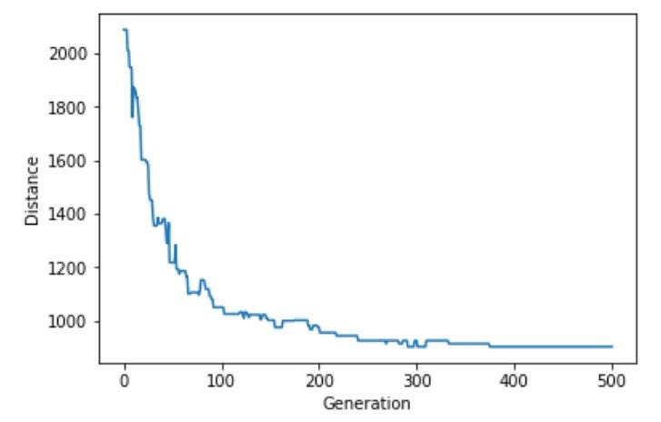
Sample output from the geneticAlgorithmPlot function
Conclusion
I hope this was a fun, hands-on way to learn how to build your own GA. Try it for yourself and see how short of a route you can get. Or go further and try to implement a GA on another problem set; see how you would change the breed and mutate functions to handle other types of chromosomes. We’re just scratching the surface here!
End notes
You can find the deployed project here.